Overview

Time estimation: 5H

Version: main

Last update: 2026-05-29

Questions:

• How does TabICL simplify the training process compared to traditional machine learning models?

Objectives:

• Learn how to create, configure, and access a VM instance in the de.NBI Cloud using SimpleVM.

• Learn basics of Streamlit syntax and deploy a trained ML model as an interactive web application.

Introduction

Machine learning projects often demand far more computational power and storage than what is typically available on local machines. Training models on large-scale datasets can quickly exceed the capabilities of personal hardware. Cloud infrastructure solves this problem by providing scalable, on-demand computing resources, making it easier to train models faster, manage larger datasets, and run reproducible workflows. Understanding how to create, configure, and access virtual machines (VMs) in the cloud is a foundational skill for scaling machine learning workflows whether for research experiments or production deployments.

In this hands-on tutorial, you will learn how to (1) create a VM instance on the de.NBI Cloud using SimpleVM; (2) preprocess and embed protein sequence dataset for training TabICL - a tabular foundation model for in-context learning on large datasets; (3) transform your trained model into an online app/service with a user interface using Streamlit.

Note

This tutorial focuses on scaling machine learning workflows in the cloud, not on the theoretical aspects of how machine learning models learn. We assume you already have basic to intermediate knowledge of model training and libraries like scikit-learn.

Prerequisites

Before you start, ensure you meet the following requirements:

• LifeScience AAI account to access the de.NBI Cloud
  • You can find instructions for registration and setup in the de.NBI Cloud Wiki
• Familiarity with the Unix commands and the SimpleVM
  • Review the previous tutorial on Unix commands or check the SimpleVM Wiki
• Basic to intermediate experience with machine learning model training and using scikit-learn library.

Preparation

Access SimpleVM instance

If you are already a member of a SimpleVM project, you can proceed to create a VM instance. If you are unfamiliar with this process, we recommend reviewing our SimpleVM tutorial and the SimpleVM Wiki for step-by-step guidance.

Instance Flavor

Ensure to select a flavor with the enough RAM and GPU, e.g. FIXME

Install the required packages

For this hands-on tutorial, we need to install the following packages:

• torch
• huggingface datasets
• tabicl
• sklearn
• pandas
• biopython
• Streamlit
• (Optional) jupyterlab

Once you have logged in your instance, install the pip following this instructions

Install `venv` and `pip3`

sudo apt update
sudo apt install python3-venv python3-pip -y
pip3 --version

Activate virtual environment and upgrade `pip`

python3 -m venv ~/mlenv
source ~/mlenv/bin/activate

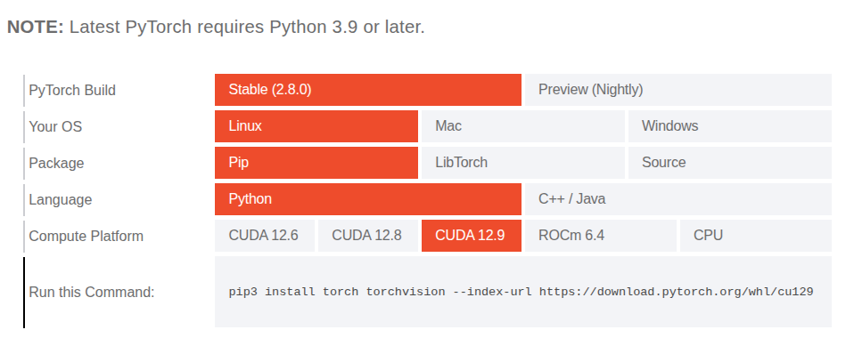
To install torch, please check the PyTorch site. Depending on your compute platform, select CPU or CUDA version and run the suggested command, e.g.:

Install the remaining packages:

pip install pandas
pip3 install -U scikit-learn
pip install tabicl # TabICL model
pip install datasets # Huggingface Datasets 
pip install streamlit # for model deployment
pip install biopython

---

Get the dataset

In this tutorial, we will use tattabio/mibig_classification_prot dataset from the Hugging Face as an example for our classification task.

The MIBiG — Minimum Information about a Biosynthetic Gene Cluster — is a community-driven standard for annotating biosynthetic gene clusters (BGCs) and their associated molecular products.

BGCs are physically linked sets of genes on a genome that collectively encode a biosynthetic pathway for producing specific metabolites, including antibiotics and antifungals, which are of great interest to the agricultural and pharmaceutical industries.

MIBiG standard provides a structured way to categorize BGCs by product type (e.g., nonribosomal peptides (NRPs), terpenes, saccharides) and enable standardized data sharing and reproducible research.

In our case, we will use this dataset to train a protein sequence classifier that predicts the class of each BGC based on sequence information.

Load and inspect the dataset

Hugging Face Datasets provides several easy ways to load the data. Navigate to Use this dataset in the dataset page and select one of the libraries:

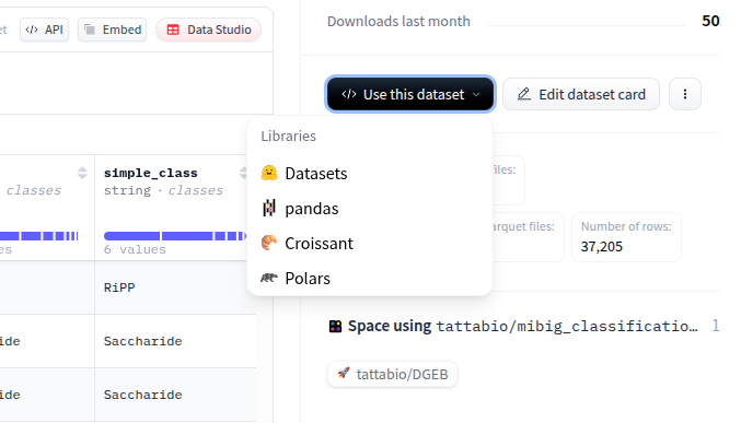
For this tutorial, we will use the datasets library from Hugging Face:

Load dataset

from datasets import load_dataset

ds = load_dataset("tattabio/mibig_classification_prot")
print(ds)

This returns the following dataset structure:

Dataset structure

DatasetDict({
    train: Dataset({
        features: ['Entry', 'Sequence', 'bgc', 'class', 'simple_class'],
        num_rows: 29992
    })
    test: Dataset({
        features: ['Entry', 'Sequence', 'bgc', 'class', 'simple_class'],
        num_rows: 7213
    })
})

The dataset comes with:

• pre-defined train/test splits for reproducible training.
• five attributes for each sample: - Entry: protein identifier - Sequence: protein sequence - bgc: biosynthetic gene cluster ID - class: detailed BGC class - simple_class: simplified, broader class categories

Convert the Hugging Face Dataset objects to Pandas DataFrames for easier manipulation using `.to_pandas()`:

train = ds["train"].to_pandas()
test = ds["test"].to_pandas()

Explore the dataset to better understand its structure before training our model

1. Handle duplicates in the Entry column for both train and test splits. Keep the same number of samples as before, but assign unique indices by creating a new column Entry_id.
2. Count how many unique classes exist in both simple_class and class. Identify which classes are most common in the dataset.

Solution

1. One way to ensure unique Entry_id values is:

   train.sort_values(by="Entry", inplace=True)
   train["Entry_id"] = train.groupby("Entry").cumcount().astype(str)
   train['Entry_id'] = train['Entry'] + '_' + train['Entry_id']
   

2. Use .value_counts() to inspect the distribution. This will reveal which classes dominate the dataset, which is critical for handling class imbalance during model training.

Pitfall #1: Class imbalance

In many biological datasets, some classes contain significantly more samples than others — known as class imbalance. This can lead to biased models that perform well on majority classes but poorly on minority ones.

Common strategies to handle class imbalance include:

• Resampling techniques
  • Oversampling minority classes (e.g., using SMOTE or random duplication).
  • Undersampling majority classes to create a more balanced dataset.
• Class weighting
  • Assigning higher weights to minority classes during training so the model pays more attention to underrepresented categories.
• Data augmentation
  • Generating synthetic samples for minority classes when biologically valid approaches are available.
• Evaluation with balanced metrics
  • Using metrics like F1-score, balanced accuracy, or Matthews Correlation Coefficient (MCC) to better assess model performance across all classes.

For this tutorial, we will use simple_class as the label because:

• it has fewer, well-distributed classes, simplifying the classification task.
• it reduces computational requirements while still demonstrating how to train and evaluate the workflow.

However, when working with more complex datasets, applying one or more of these techniques is recommended to improve model robustness.

Extract protein embeddings using gLM2

To train our classifier, we first need to convert protein sequences into numerical representations, i.e embeddings. Embeddings capture biological and contextual information from sequences, enabling the machine learning model to learn patterns effectively. For this, we use the tattabio/gLM2_650M_embed, a genomic language model fine-tuned specifically for functional annotation task.

gLM papers and platforms

For more information regarding the model, please read the following papers:

• Gaia: A Context-Aware Sequence Search and Discovery Tool for Microbial Proteins
• The OMG dataset: An Open MetaGenomic corpus for mixed-modality genomic language modeling
• Genomic language model predicts protein co-regulation and function

Also, if you are interested in functional annotation of the protein sequences, check the Gaia annotator and SeqHub from the Tattabio.

Step 1: Import the required packages

Code-in

import torch
from torch.utils.data import DataLoader, Dataset
from transformers import AutoModel, AutoTokenizer
import pandas as pd

Packages description

• torch and torch.utils.data: for tensor operations and data batching.
• transformers: for loading the gLM2 model and tokenizer.
• pandas: for handling dataframes.

Check if GPU is available:

import torch
print(torch.cuda.is_available())  # should return True on GPU-enabled instances

Embedding thousands of sequences is computationally intensive. While CPUs are versatile, they process data sequentially and can be orders of magnitude slower.

GPUs, on the other hand, are optimized for parallel computation. They enable processing many sequences at once, significantly speeding up the embedding step and making large-scale workflows practical.

Step 2: Load the model and tokenizer

Code-in

model_name = 'tattabio/gLM2_650M_embed' # path of the pre-trained model hosted on Hugging Face Hub
device = "cuda" if torch.cuda.is_available() else "cpu" # check if a GPU is available for faster computation; otherwise, run on CPU

model = AutoModel.from_pretrained(model_name, torch_dtype=torch.bfloat16, trust_remote_code=True).cuda()
tokenizer = AutoTokenizer.from_pretrained(model_name, trust_remote_code=True)

Description

• torch_dtype=torch.bfloat16 – specifies the data type for model weights. Using bfloat16 reduces memory usage and speeds up computation on GPUs without significantly sacrificing precision.
• trust_remote_code=True – allows execution of custom code provided by the model repository (required when models have custom architectures or tokenizers). Only use this flag with trusted sources.
• .cuda() – moves the model to the GPU, enabling faster computation for embedding generation.
• AutoTokenizer.from_pretrained(...) – loads the tokenizer associated with the model, ensuring proper tokenization of sequences for embedding generation.

Step 3: Build a custom `Dataset`

We define a small ProteinDataset class to store sequences and their IDs. This will let the DataLoader efficiently iterate through the dataset in batches:

Code-in

class ProteinDataset(Dataset):
   def __init__(self, seq_dict):
       self.keys = list(seq_dict.keys())
       self.sequences = list(seq_dict.values())

   def __len__(self):
       return len(self.keys)

   def __getitem__(self, idx):
       return self.keys[idx], str(self.sequences[idx])

Step 4: Collate function for tokenization

The collate function batches sequences together and tokenizes them dynamically. By padding (i.e., adding special tokens to shorter sequences so all sequences in a batch have the same length) and truncating (i.e., shortening sequences that exceed the maximum length) sequences to the same length within each batch, the model can process them efficiently.

Padding and Truncation

For a comprehensive explanation of padding and truncation strategies, refer to the Hugging Face documentation.

Code-in

def collate_fn(batch):
   keys, sequences = zip(*batch)
   tokens = tokenizer(
       list(sequences),
       padding=True,
       truncation=True,
       return_tensors='pt'
   )
   return keys, tokens

Step 5: Create a `DataLoader`

The DataLoader handles batching, shuffling (if needed), and efficient data loading. Here, we use a batch_size of 32 — a good starting point for GPUs with moderate memory. Adjust the size depending on your GPU capacity:

Code-in

train_dc = train.set_index("Entry_id")["Sequence"].to_dict()
train_dataset = ProteinDataset(train_dc)

train_loader = DataLoader(
   train_dataset,
   batch_size=32,  # adjust based on GPU memory
   shuffle=False,
   collate_fn=collate_fn
)

Step 6: Generate embeddings

Iterate over the DataLoader, move each batch to the GPU, and extract embeddings from the model.

Code-in

embeddings = {}

model.eval()
with torch.no_grad():
   for keys, tokens in tqdm(train_loader, desc="Embedding Sequences"):
       tokens = {k: v.to(device) for k, v in tokens.items()}
       outputs = model(tokens["input_ids"]).pooler_output.cpu()
       for k, emb in zip(keys, outputs):
           embeddings[k] = emb.to(torch.float32)

torch.save(embeddings, "train.pt")          

Description

Here,

• model.eval() ensures we are in inference mode (no gradients computed, faster processing).
• torch.no_grad() disables gradient tracking, reducing memory usage.

Repeat the last step for the test split and save the embeddings.

---

---

---

What to learn next?

Explore alternative approaches to deploy your trained model on the cloud:

• Deploy the model on cloud with FastAPI

Key Points

• Streamlit allows rapid creation of user-friendly web apps for deploying models and sharing results.

Supported by: